Learning the Language of Rain

Neural networks as entropy sinks in simulations of real-world phenomena

Huawei’s Pangu LLM is a bit of an oddity. It’s one of the biggest models publicly available (200 billion parameters), and - according to its makers - can do almost anything. In practice, however, it does barely anything because no one is using it. Upon conducting a rigorous large-n enquiry (asking a few people I know in the industry whether they or anyone they know have used it) the results included blank stares at best and ridicule at worst. It is widely known, for example, that Pangu is under-trained for text generation (and we’ll get back to this intriguing fact later), and Ernie Bot (文心一言) is far better at producing Chinese texts.

So if text isn’t Pangu’s thing, what about some of its other skills?

Weather prediction is the main one - Huawei recently did a press blitz about a Nature paper published by its researchers showing that that Pangu’s predictions were surpassing current EU standard models (the European Centre for Medium-Range Weather Forecasts’ Integrated Forecasting System or IFS) for accuracy. And indeed, if you look at its results, they’re… not bad. One may even go so far as to say they are pretty decent.

Image courtesy of the Pangu team

Its predictions are slightly better than IFS, though a component of this may be over-fitting on the measure of assessment used. You can read a pretty balanced evaluation of the Pangu paper by the ECMWF here. In fact, Pangu’s principal advantage is that it completes its calculations much faster and at a lower cost than conventional physics-based weather models. The IFS and models like it are essentially based on mathematical approximations of real world processes - if it’s cloudy in Brighton and there’s a South wind, you can reasonably predict that it’ll soon be cloudy in London. This process can be copied in low-res by splitting the map up into cubes and then using a set of partial differential equations to describe how the various types of weather you’re interested in travel from cube to cube - a very slow and compute-intensive process.

I stole this from a Colorado State University PowerPoint but sadly I have no idea who the author was.

To give you an idea, here are the processes that need to be factored in for every grid cube in the IFS’s “moist physics” model:

Image courtesy of the ECMWFS

Information on roughly 35-45 parameters, some of which are measured, others estimates or internal to the model, are fed through one or more of three sets of rules (relating to relative humidity, cloud and precipitation) for each cube of geography covered, thus describing the relationship between that cube’s previous stats, those of its neighbours and its nine output variables (cloud fraction, specific humidity etc.).

Pangu, for its part, tracks 69 “factors” - five upper air variables at 13 pressure levels, plus four surface variables. Rather than using a pre-established set of equations to transform them into outputs, it simply dumps them into a deep neural net and trusts the AI to spot the patterns between the values of one cube and those of the others. And, as mentioned above, it’s a little better at predicting future changes than some traditional models, while also being much faster (a very important factor in weather prediction for obvious reasons).

But here’s where it gets interesting: Google’s much smaller Metnet and Metnet 2 models (225 million parameters) are also beating industry standard forecasting methods – and seemingly by a more significant margin (around 50%) - taking as their input pictures of rain clouds. Here’s an example:

According to Google, this is a suite of actual inputs used.

I should immediately qualify this by pointing out that it is not a direct one-for-one comparison of the two models. Not only did the two teams use different measures of accuracy, impeding any attempt at like-for-like assessment, but Metnet only predicts rain while Pangu predicts almost everything but rain, Pangu specialises in medium lead times and Google in shorter ones, etc. etc.[1]. Nevertheless, Google’s remarkable performance raises a number of interesting questions.

The performance of a weather model can be described in terms of two things:

1. The spread of the results over multiple runs;

2. How close the centre of this spread is to whatever the actual weather is at the time.

The latter is basically a reflection of the accuracy of the data points we have and the maths we use to describe their evolution, and tells us how likely we are to get any given prediction right. The former is describes the level of divergence between all of the model outputs (either as a result of deliberately adding noise to the input data and rerunning the model multiple times to create an ensemble forecast, or in the form of sequential individual forecasts’ positions relative to the actual outcome that followed) plus the real world outcome. It is a reflection of model entropy[2] and tells us how likely we are to get any given prediction wrong.

If the red dot here represents the real-world weather and the black ones the models’ predictions (whether in the course of a single ensemble forecast, or as relative positions over time), then both of the models below are pretty good, though they will likely give very different outputs on any given run. In the one on the left the cluster is a little off, but the outlying predictions are also much closer to the actual outcome, meaning that you’re less likely to be very wrong. In the one on the right, the centre of the cluster is closer to the true outcome, but it’s harder to work out where this centre is on account of the dispersal of the points.

Either an actual outcome and the ensemble forecast that preceded it, or a series of actual outcomes and the relative coordinates of the non-ensemble predictions that preceded them. Meteorologists describe the diffusion of the points as uncertainty or spread.

Obviously, the perfect model would be one that produced a tight cluster of points centred in the vicinity of the real-world outcome - high skill and low spread, as the meteorologists put it. There are plenty of steps that can be taken to optimise along both dimensions, but eventually you hit a wall at which point adding variables to your model provides additional data (helping you to centre your cluster better) but also more entropy (making your cluster more dispersed) - what you gain on one measure you simultaneously lose on the other.

The tendency for more complex models to produce greater uncertainty has been observed regularly. For example, here you can see here that two sets of parameters (represented in green here) that contribute barely any model uncertainty when applied singularly (M_S and M_A,L) suddenly start generating huge amounts when combined (M_A,Q):

Impressive, right?

This is often analysed as a purely practical problem - a reflection of the fact that less informative variables tend to be added last, and that they are occasionally so uninformative that they end up making the model less accurate rather than more. The example above, however, seems to hint at more than that - after all, all of its variables were perfectly fine until we combined them. Errors are not the only source of model entropy however. There are two others that are likely to be of interest to us here:

1. Overfitting: In the case of artificial neural networks at least, overparametrised[3] models have a tendency to get all bored and trigger-happy and use their spare capacity to identify relationships that don’t actually exist, leading to increased output variance[4].

2. Omissions: There plenty of processes going on in the real world that affect the model outcomes but which aren’t described by the variables we have (global warming, for example, or the effect of the Covid lockdown on cloud cover). This is why there is no way to eliminate model entropy entirely without building an exact atom-for-atom replica of our own universe within the simulation. It also means that even a model with perfect data and design will get almost every interaction it simulates slightly wrong, and do so in unpredictable ways, since the errors are being produced by real-world phenomena that do not exist in the model world, rather than by known flaws in the simulated phenomena.

An analogy might be an image of a drone pilot attempting to track a skier for the length of a two-minute downhill run. Every ten seconds his hand is given a random buffet. This may push the drone back or forwards on its present path, or shift it right, left, up or down.

This excellent diagram was made by the ECMWF.

The exercise is then repeated with his hand receiving two buffets every ten seconds. The drone won’t always end up further from the skier, but over 10,000 runs the circle incorporating the coordinates of its final positions will be wider - just as if the skier had continued for four minutes instead of two.

While it’s difficult to compare the number of interactions going on per second in the IFS and Pangu models (partly because we have no idea what’s going on inside Pangu’s black box), my guess would be that Pangu’s cubes are interacting more with one another per iteration than IFS’s are, simply because the IFS system privileges relations between nearest neighbours while the Pangu one uses a relative positional bias approach (which can also emphasise other relationships if they seem important).

This means that even if the Pangu team’s high-context pattern-recognition approach produces a more nuanced and contingent description of the interactions between variables than the mechanistic and inflexible systems of partial differential equations used in conventional physics-based models, by simulating more interactions per iteration it is likely that it is simultaneously injecting more entropy into the model. This means that the centre of its results cluster is probably closer to the real-world outcome, but that it is harder to tell where that centre is. The model is being forced to fight its own dissipation with every iteration.

Possibly going some way to confirm this, Pangu’s ensemble spread-skill correlation seems lower than that of the IFS ensemble model.

Skill spread ratios for Pangu and IFS (the latter courtesy of the WeatherBench 2 team, the former from the Pangu Nature paper). Unfortunately, there are several different ways to calculate this measure, and I am not sure which the Pangu team used, so this is not necessarily conclusive.

While this measure of model reliability is a controversial one, the reduced correlation may imply that Pangu has added some accuracy but even more spread, as compared to IFS. Of course, it’s also important to bear in mind that Pangu is also faster and more computationally efficient, meaning that this can be corrected for by creating an ensemble forecast with more members (i.e. running the model more times). The tldr is that what you gain on the swings you lose on the roundabouts, and then finally claw back on the GPUs.

Having considered all of this information, you might suppose it to be the key to Metnet’s comparatively high performance. Normally the best predictor of a variable’s future values is its past values, so one would tend to assume that rain is simply the most significant predictor of rain and that adding others to the simulation contributes more entropy than predictive power. The problem with this, however, is that rain is not a good predictor of rain. In fact, it’s such a bad predictor that a lot of traditional models don’t include it at all, and instead rely upon temperature, wind speed, relative humidity and a grab-bag of geographical variables[5]. This means that Metnet is not just producing better outputs, it is producing them using a variable with such a weak predictive relationship to the desired result that it was once regarded as basically useless.

The only possible explanation we are left with is that the rain itself is somehow encoding the factors that went into producing it, but it is doing so in a non-human-readable format. This means that from the model’s perspective, the images constitute only one variable (thus minimising interactions and hence entropy accretion), but they can be unpacked in such a way as to provide information on all of the factors that went into producing them - the wind speed data, humidity levels etc. are compressed within the rain cloud images.

To simplify somewhat (and you can skip this paragraph if you don’t care about the maths), imagine two models. Each is trying to calculate an output A, which is a function of three inputs: B, C and D. Each of these inputs interact with each other and with an unknown number of unknown inputs, U, with the whole kit and caboodle also suffering from measurement inaccuracies and any flaws present in the model maths, creating an entropy term in every interaction - Η. In the first case the model is given data relating to the variables for which data is available and which are known to be contributors of information about A (that is B, C and D, but not U, because we have no data on U), making A^t0 a function of (B^t-1+Η)+(C^t-1+Η)+(D^t-1+Η)+H. Each variable carries with it an entropy term that is the result of measurement inaccuracies and model flaws, plus that variable’s interactions with the unknown variables, which themselves contribute entropy but no predictive power. In the second case, the model receives only A^t-1 as an input, with A^t0 being a function of A^t-1+Η (with H here representing only model flaws and measurement inaccuracies). In this case, however, the model is able to decode A^t-1 as a representation not just of B^t-2, C^t-2 D^t-2, but also U^t-2. I.e. it receives the same information as before - albeit with a one-iteration lag, but also information about the unknown variables that was omitted from the first model. However, because these interactions are not actually simulated by the model they add no extra Η. Indeed, given a flawless model and no measurement inaccuracies, Η would be entirely eliminated by the encoding of U.

This is possible thanks to the way in which neural networks process information, functioning as extremely efficient lossless compressors.

In information theory, entropy and information are synonymous, an idea that is confusing at first glance, but easy to grasp once you realise that the more different A is from B, the more bits will be required to describe this difference. (Thus tying in the information theory definition of entropy with the probability-based one we used above - the more model iterations diverge, the more information is required to describe this divergence.) However, this relationship is not always precisely linear, particularly in natural language contexts. More or fewer bits may be required to convey information depending on the language being used, and in many cases the number of bits required is entirely unrelated to the characteristics of the phenomena being described. Thus, for example, in English fewer bits are required to describe a cat (three letters) than a hydrogen atom (12 letters and a space). However, if we reduce the hydrogen atom to its chemical symbol - H - the same information is conveyed in a much compressed form, and the hydrogen atom is once again smaller and less complex than the cat.

The extent to which compression is possible depends partly on the number of letters in the language at hand. In English only 26 one-letter words are possible, 650 two-letter words, 15,600 three-letter words etc. If we use modern Japanese katakana, however, we have 73 possible one-letter words, 5,256 possible two-letter words, and a massive 373,176 three-letter words available to us. If a language is limited to words below a certain length (million-character words are not a feasible proposition, whatever the Germans may say), then the more letters it has, the more concepts it will be able to describe precisely using one-word terms. Conversely, if a language is limited in both the number of letters it has and the length of its possible words, it will be forced to concatenate multiple words even to describe relatively simple concepts and still tend to suffer from imprecision (Toki Pona is a real-world example of this, albeit at the level of words rather than letters).

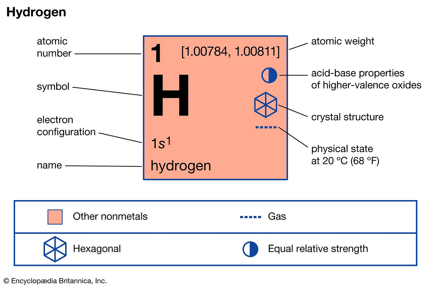
However, the level of compression is also a function of the processing medium. For me, with my residual memories of high school chemistry, H can be unpacked into a hydrogen atom. For an illiterate Yanomami tribesman in Brazil, it is simply three lines, while a chemistry professor will be capable of extracting a whole world of information from the same letter:

Images all from Google. I am not a chemist but these look impressive as hell and most likely hard to compress.

I am a more efficient compressor of H related information the Brazilian tribesman, but far less efficient than the chemistry professor. (Conversely, the Yanomami is doubtless a much better compressor of jungle survival information than either of us.) Imagine a scenario in which the three of us were asked to transmit the following description from Wikipedia to an educated recipient in a neighbouring room:

“Hydrogen can be produced by pyrolysis of natural gas (methane). Methane pyrolysis is accomplished by passing methane through a catalyst. Methane is converted to hydrogen gas and solid carbon.”

The Yanomami would be obliged to memorise the message stroke by stroke. For him it is already as compressed as it will ever get, and any attempt to skip a stroke or two would reduce the fidelity of the transmission. I have just enough of an understanding of what’s going on here (and the language in which it is written) that I could manage to summarise it accurately in fewer words: “Methane pyrolysis uses a catalyst to produce hydrogen gas and solid carbon from methane gas.” The chemistry professor could go one better: “CH4(g) → C(s) + 2 H2(g)”

The professor can extract more information from fewer bits (and, similarly, compress more information into a smaller number of bits) because H is already tied into a multitude of other concepts in his brain. In other words, our relative ability to compress information is a function of the dimensionality of the data upon which we were pre-trained. For the professor, H is a high-dimensional data object, not because he is receiving higher-dimensional input data than the rest of us, but because he arrived with the requisite dimensions pre-loaded and simply had to slot the letter provided into the analysis space he had prepared for it[6].

Neural networks take advantage of both of the above-mentioned phenomena - long alphabets allowing for high specificity and front-loading dimensionality by pre-training. Thus they are able to parse information inaccessible to humans and process it efficiently. In the case of Metnet, every model parameter can be understood as a letter in the model’s language, meaning that each image it is trained on becomes a new word in its vocabulary, a precise description of a given rainstorm and the circumstances that produced it - one that would require pages of natural language text to replicate. When shown in sequence, such images become a sentence in which it is relatively easy for the model to predict the next words[7].

Image courtesy of Jason Weingart: https://en.wikipedia.org/wiki/File:Evolution_of_a_Tornado.jpg

By using a neural network to process your data, you offload the descriptive complexity onto the language used and the analytic device employed to parse it. We have reduced the number of input variables to one, but the information provided by the other variables has not disappeared, it is simply being stored somewhere else, thereby squirreling away a corresponding quantum of entropy. In other words, the efficient high-dimensional parametrised memory system created by a neural network allows it to extract detailed information about multiple variables from a single input variable, thus permitting it to serve as an entropy sink when simulating real-world phenomena.

However, just as rain images can encode data on temperature, wind speed and humidity, so the Huawei and Google approaches to this problem encode data on their respective corporate strategies. Huawei – a hardware firm at base – has minimal interest in AI beyond predictive maintenance and self-driving cars, but has clearly been ordered by the Party to find muscular communist uses for LLMs to make the Americans look like effete and impractical time-wasters to the rank and file. This not being their core business, they have accordingly put in the bare minimum required to allow CEO Zhang Ping’an to brag in public that “we don’t write poems, we do things” (it sounds catchier in Chinese), before going back to his batteries. Putting as little work into this as they could get away with, they replaced the partial differential equations in a conventional weather model with a deep neural net and declared victory. Job postings on the Huawei site seem to confirm as much – the company’s major need for AI specialists lies in hardware-related tasks, with only one or two low-level postings relating to flood modelling in Germany. The under-training of the text generation version of Pangu mentioned above can be read as a manifestation of a similar phenomenon: if Pangu were fully pre-trained Huawei would then be forced to divert resources to making sure that it would say only politically correct things. The only sensible solution is to ensure that it will under-perform in this particular field and find another - say, weather prediction - in which to claim superiority. The Party bosses are happy and minimal time has been wasted on non-core tasks. Everyone’s a winner (except, presumably Baidu, which has been lumbered with the unenviable task of training an LLM such that it will never say anything that can be interpreted as disagreeing with the party line).

The Google engineers, by contrast, seem to be making a genuine effort to not simply build a weather model with AI in, but to build an AI weather model, beginning from first principles and redefining our understanding of what weather models are and can be. The design of Metnet 2 seems to show that entropy minimisation is a deliberate strategy on their part – they are not simply using rain pictures because they have a lot of them. Metnet 2’s base state was modified to incorporate 612 other variables, but – unlike Pangu - it does not track their evolution over time. They simply provide as much data as they are capable of at t=0 before dropping out of the model. Because they do not increase the total number of interactions within the simulation, they also contribute little entropy – making the model better without also making it worse. Not only is Google’s approach achieving impressive results, it’s giving us new ways to think about the problem of simulating physical systems in general.

All of which may sound like a criticism of Pangu, which is not intended. As mentioned above, while Pangu’s predictions probably have a wider spread, this can be compensated for by creating ensemble forecasts with more members (i.e. rerunning the simulation more times with slightly perturbed input data each time), something that its lower compute requirements allow it to do quite easily. Moreover, the fact that it manages to do a decent job despite being engulfed in corporate indifference gives a hint of its true capabilities. Now we just need to work out what it’s really good at.

Thanks to David, EpsilonPraxis, Jacopo and Silap for their assistance with this piece.

---

[1] It should nevertheless be noted that what Metnet is doing does not fall under the traditional definition of nowcasting (predicting rainfall up to either two or six hours ahead, depending on who you ask), though other Google teams have used similar methods in dealing with nowcasting challenges.

[2] A nice summary of the various definitions of entropy can be found here. “In classical physics, the entropy of a physical system is proportional to the quantity of energy no longer available to do physical work. Entropy is central to the Second Law of thermodynamics, which states that in an isolated system any activity increases the entropy; in quantum mechanics, von Neumann entropy extends the notion of entropy to quantum systems by means of the density matrix. In probability theory, the entropy of a random variable measures the uncertainty about the value that might be assumed by the variable; in information theory, the compression entropy of a message (e.g., a computer file) quantifies the information content carried by the message in terms of the best lossless compression rate, in the theory of dynamical systems, entropy quantifies the exponential complexity of a dynamical system or the average flow of information per unit of time; in sociology, entropy is the natural decay of structure (such as law, organization, and convention) in a social system; and in the common sense, entropy means disorder or chaos.” I am using it in the probability sense here, on the understanding that entropy is assessed at the level of every possible iteration of a simulation plus the real world events it is attempting to replicate. Meteorologists tend to refer to this as uncertainty or spread, but I will be drawing links with the information theory definition later in the piece and hence have preferred terminological unity.

[3] Irritatingly, overparametrisation as used in regular model design does not function in exactly the same way as in machine learning, referring to something closer to overspecification. Similarly, in climate modelling “uncertainty” is often used to refer to something that is almost the direct opposite of uncertainty in weather modelling - the number of variable combinations that can be used to achieve broadly similar results.

[4] My thanks to Silap for pointing this out.

[5] This is partly on account of the extreme localisation/short duration of rainfall, which tends to happen at too small a scale for the models to resolve, partly it is simply not a very good predictor.

[6] Coincidentally, Yan LeCun just tweeted something along these lines: https://twitter.com/ylecun/status/1701315853550014843 and it may help to explain why some overparametrised (in the AI sense) models still don’t overfit - more information is being given to them than the data, taken at face value, would suggest. It also feels like the whole thing should tie into Taken’s embedding theorem somehow but I do not know anywhere near enough about topology to be able to make the link.

[7] Or, as Google’s team put it, “MetNet-2 appears to emulate the physics described by Quasi-Geostrophic Theory, which is used as an effective approximation of large-scale weather phenomena. MetNet-2 was able to pick up on changes in the atmospheric forces, at the scale of a typical high- or low-pressure system (i.e., the synoptic scale), that bring about favorable conditions for precipitation, a key tenet of the theory.”